R入門
線形回帰分析(朝倉書店)
最終更新:
r-intro
目次
- 目次
- 最小二乗法による正規線形回帰モデルのパラメーターの推定(pp.14-17)
- 例2.2 風速と直流発電量(pp.62-67)その1
- 例2.2 風速と直流発電量(pp.62-67)その2
- 例2.3 直流発電量の予測と予測区間(pp.72-75)
- 例2.4 年齢と最高血圧(pp.75-82)その1
- 例3.3 配達時間 (1),(2)(pp.106-113)
- 例3.3 配達時間 (1),(2)(pp.106-113)※lm関数使用版
- 例3.3 配達時間 (3)(pp.113-114)
- 例3.4 平均勤続年数と所定内賃金(pp.116-118)
- 貨幣賃金率変化率の回帰モデルの推定(pp.119-120)
最小二乗法による正規線形回帰モデルのパラメーターの推定(pp.14-17)
表1.1のデータのファイルをカレントディレクトリに置いて行うこと。
> dtf <- read.csv("table1_1.csv", header = TRUE)
> xxi <- log(as.double(dtf$NIC))
> yyi <- log(as.double(dtf$CO))
> n <- nrow(dtf)
> ssxx <- sum(xxi)
> ssyy <- sum(yyi)
> ssxx2 <- sum(xxi ^ 2)
> ssyy2 <- sum(yyi ^ 2)
> ssxxyy <- sum(xxi * yyi)
> xxim <- ssxx / n
> yyim <- ssyy / n
> ssx2 <- ssxx2 - ssxx ^ 2 / n
> ssy2 <- ssyy2 - ssyy ^ 2 / n
> ssxy <- ssxxyy - ssxx * ssyy / n
> bh <- ssxy / ssx2
> ah <- yyim - bh * xxim
> yyhi <- ah + bh * xxi
> ei <- yyi - yyhi
> ri <- ei / yyi * 100
> ai2 <- ei ^ 2 / sum(ei ^ 2) * 100
> #
> cat(sprintf("β^ = %.6f\n", bh))
β^ = 1.054475
> cat(sprintf("α^ = %.6f\n", ah))
α^ = 2.663670
> s <- sprintf("%7.5f %7.5f %8.5f %6.2f %5.2f", yyi, yyhi, ei, ri, ai2)
> for (i in 1:n) cat(sprintf("%2d %s\n", i, s[i]))
 1 2.61007 2.50463  0.10544   4.04  2.49
 2 2.80940 2.72511  0.08429   3.00  1.59
 3 3.15700 3.41028 -0.25328  -8.02 14.35
 4 2.32239 2.24138  0.08101   3.49  1.47
 5 1.68640 1.69746 -0.01106  -0.66  0.03
 6 2.70805 2.70503  0.00302   0.11  0.00
 7 2.19722 2.37428 -0.17706  -8.06  7.01
 8 2.50960 2.60958 -0.09998  -3.98  2.24
 9 2.79117 2.78317  0.00799   0.29  0.01
10 2.73437 2.68455  0.04982   1.82  0.56
11 2.56495 2.67416 -0.10921  -4.26  2.67
12 2.66723 2.55257  0.11466   4.30  2.94
13 2.30259 2.07093  0.23166  10.06 12.00
14 2.32239 2.40167 -0.07929  -3.41  1.41
15 2.25129 2.34616 -0.09487  -4.21  2.01
16 0.40547 0.51231 -0.10684 -26.35  2.55
17 2.91777 2.90737  0.01040   0.36  0.02
18 2.53370 2.74482 -0.21113  -8.33  9.97
19 2.86220 2.62062  0.24158   8.44 13.06
20 1.58924 1.74891 -0.15968 -10.05  5.70
21 2.76632 2.67416  0.09216   3.33  1.90
22 2.14007 2.14245 -0.00238  -0.11  0.00
23 2.36085 2.27239  0.08846   3.75  1.75
24 2.63189 2.68455 -0.05266  -2.00  0.62
25 2.70136 2.45441  0.24695   9.14 13.64
> #
> plot(xxi, yyi, xlim = c(-2, 0.7), ylim = c(0.4, 3.5), pch = 20)
> idx <- order(xxi)
> lines(xxi[idx], yyhi[idx])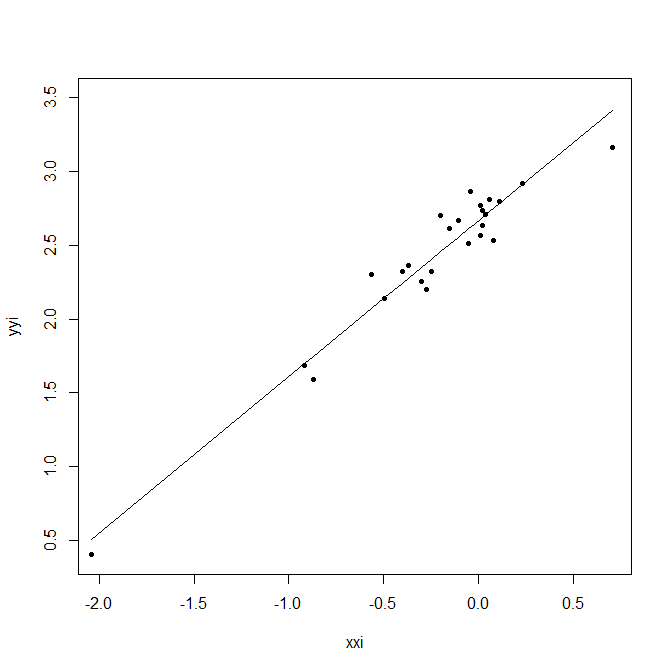
例2.2 風速と直流発電量(pp.62-67)その1
p.63に掲載されている3つのモデルについて、それぞれlm関数を使って計算している。表2.1(p.62)の値をCSV形式で入力した table2_1.csvをカレントディレクトリに置いておくこと。
> dtf <- read.csv("table2_1.csv", header = TRUE)
> xxi <- as.double(dtf$WV)
> yyi <- as.double(dtf$DC)
> # 式(2.28)
> r1 <- lm(yyi ~ 1 + xxi)
> print(summary(r1))
Call:
lm(formula = yyi ~ 1 + xxi)
Residuals:
     Min       1Q   Median       3Q      Max
-0.59869 -0.14099  0.06059  0.17262  0.32184
Coefficients:
            Estimate Std. Error t value Pr(>|t|)
(Intercept)  0.13088    0.12599   1.039     0.31
xxi          0.24115    0.01905  12.659 7.55e-12 ***
---
Signif. codes:  0 ‘***’ 0.001 ‘**’ 0.01 ‘*’ 0.05 ‘.’ 0.1 ‘ ’ 1
Residual standard error: 0.2361 on 23 degrees of freedom
Multiple R-squared:  0.8745,    Adjusted R-squared:  0.869
F-statistic: 160.3 on 1 and 23 DF,  p-value: 7.546e-12
> # 式(2.29)
> r2 <- lm(yyi ~ 1 + log(xxi))
> print(summary(r2))
Call:
lm(formula = yyi ~ 1 + log(xxi))
Residuals:
     Min       1Q   Median       3Q      Max
-0.31619 -0.07685  0.02395  0.11139  0.23029
Coefficients:
            Estimate Std. Error t value Pr(>|t|)
(Intercept) -0.83036    0.11083  -7.493  1.3e-07 ***
log(xxi)     1.41677    0.06234  22.728  < 2e-16 ***
---
Signif. codes:  0 ‘***’ 0.001 ‘**’ 0.01 ‘*’ 0.05 ‘.’ 0.1 ‘ ’ 1
Residual standard error: 0.1376 on 23 degrees of freedom
Multiple R-squared:  0.9574,    Adjusted R-squared:  0.9555
F-statistic: 516.6 on 1 and 23 DF,  p-value: < 2.2e-16
> # 式(2.30)
> r3 <- lm(yyi ~ 1 + I(1 / xxi))
> print(summary(r3))
Call:
lm(formula = yyi ~ 1 + I(1/xxi))
Residuals:
     Min       1Q   Median       3Q      Max
-0.20547 -0.04940  0.01100  0.08352  0.12204
Coefficients:
            Estimate Std. Error t value Pr(>|t|)
(Intercept)   2.9789     0.0449   66.34   <2e-16 ***
I(1/xxi)     -6.9345     0.2064  -33.59   <2e-16 ***
---
Signif. codes:  0 ‘***’ 0.001 ‘**’ 0.01 ‘*’ 0.05 ‘.’ 0.1 ‘ ’ 1
Residual standard error: 0.09417 on 23 degrees of freedom
Multiple R-squared:   0.98,     Adjusted R-squared:  0.9792
F-statistic:  1128 on 1 and 23 DF,  p-value: < 2.2e-16
例2.2 風速と直流発電量(pp.62-67)その2
pp.64-67に掲載されている、p.23の式(2.30)による結果を流れに沿って計算している。表2.1(p.62)の値をCSV形式で入力したtable2_1.csvをカレントディレクトリに置いておくこと。
> dtf <- read.csv("table2_1.csv", header = TRUE)
> xxi <- as.double(1 /dtf$WV)
> yyi <- as.double(dtf$DC)
> n <- nrow(dtf)
> k <- 2
> ssxx <- sum(xxi)
> ssyy <- sum(yyi)
> ssxx2 <- sum(xxi ^ 2)
> ssyy2 <- sum(yyi ^ 2)
> ssxxyy <- sum(xxi * yyi)
> xxm <- mean(xxi)
> yym <- mean(yyi)
> ssx2 <- ssxx2 - ssxx ^ 2 / n
> ssy2 <- ssyy2 - ssyy ^ 2 / n
> ssxy <- ssxxyy - ssxx * ssyy / n
> bh <- ssxy / ssx2
> ah <- yym - bh * xxm
> ssyh2 <- bh * ssxy
> r2 <- ssyh2 / ssy2
> sse2 <- ssy2 - ssyh2
> s2 <- sse2 / (n - k)
> s <- sqrt(s2)
> sah2 <- s2 * (1 / n + xxm ^ 2 / ssx2)
> sah <- sqrt(sah2)
> ta <- ah / sah
> sbh2 <- s2 / ssx2
> sbh <- sqrt(sbh2)
> tb <- bh / sbh
> yyhi <- ah + bh * xxi
> ei <- yyi - yyhi
> ri <- 100 * ei / yyi
> ai2 <- 100 * (ei ^ 2 / sse2)
> sh2 <- sum(ei ^ 2) / n
> print(ah)  # 推定されたパラメーター α^
[1] 2.97886
> print(bh)  # 推定されたパラメーター β^
[1] -6.934547
> print(sh2)  # 誤差項の分散の最尤推定量 σ^^2
[1] 0.008158786
> dtf <- data.frame(yyi, yyhi, ei, ri, ai2)
> colnames(dtf) <- c("DC", "DC推定値", "残差", "誤差率(%)", "平方残差率(%)")
> print(dtf)
      DC  DC推定値         残差    誤差率(%) 平方残差率(%)
1  1.582 1.5919507 -0.009950703  -0.62899514   0.048544719
2  1.822 1.8231023 -0.001102282  -0.06049844   0.000595689
3  1.057 0.9392874  0.117712578  11.13647849   6.793290635
4  0.500 0.4105093  0.089490699  17.89813971   3.926361222
5  2.236 2.2854054 -0.049405439  -2.20954556   1.196696381
6  2.386 2.2639584  0.122041615   5.11490423   7.302143226
7  2.294 2.2527296  0.041270439   1.79906010   0.835050285
8  0.558 0.7052381 -0.147238090 -26.38675451  10.628569260
9  2.166 2.1279955  0.038004532   1.75459519   0.708117342
10 1.866 1.8603848  0.005615206   0.30092206   0.015458445
11 0.653 0.5876369  0.065363052  10.00965576   2.094590369
12 1.930 1.8868055  0.043194527   2.23805841   0.914727865
13 1.562 1.4713499  0.090650121   5.80346482   4.028758432
14 1.737 1.7832486 -0.046248561  -2.66255390   1.048650839
15 2.088 2.0417592  0.046240820   2.21459864   1.048299802
16 1.137 1.0525970  0.084402980   7.42330521   3.492609407
17 2.179 2.0954783  0.083521654   3.83302682   3.420051394
18 2.112 2.1908434 -0.078843429  -3.73311692   3.047652653
19 1.800 1.9882106 -0.188210552 -10.45614178  17.366903572
20 1.501 1.7064662 -0.205466164 -13.68861852  20.697366094
21 2.303 2.2168220  0.086177997   3.74198856   3.641055032
22 2.310 2.2990026  0.010997410   0.47607833   0.059294615
23 1.194 1.2875072 -0.093507161  -7.83142048   4.286710893
24 1.144 1.2232786 -0.079278565  -6.92994450   3.081385381
25 0.123 0.1484327 -0.025432682 -20.67697705   0.317116449
> # 図2.8と2.9の作成
> png("fig2_8.png", width = 512, height = 512)
> plot(1 / xxi, yyi, xlim = c(2, 11), ylim = c(0, 2.5), xlab = "WV", ylab = "DC", pch = 20)
> idx <- order(1 / xxi)
> lines(1 / xxi[idx], yyhi[idx])
> dev.off()
null device
          1
> png("fig2_9.png", width = 512, height = 512)
> plot(xxi, yyi, xlim = c(0.09, 0.42), ylim = c(0, 2.5), xlab = "1 / WV", ylab = "DC", pch = 20)
> idx <- order(xxi)
> lines(xxi[idx], yyhi[idx])
> dev.off()
null device
          1
例2.3 直流発電量の予測と予測区間(pp.72-75)
> dtf <- read.csv("table2_1.csv", header = TRUE)
> n <- nrow(dtf)
> xxi <- 1 / dtf$WV
> yyi <- dtf$DC
> k <- 2
> degf <- n - k
> xxm <- mean(xxi)
> yym <- mean(yyi)
> ssx2 <- sum((xxi - xxm) ^ 2)
> ssxy <- sum((xxi - xxm) * (yyi - yym))
> bh <- ssxy / ssx2
> ah <- mean(yyi) - bh * xxm
> sse2 <- sum((yyi - (ah + bh * xxi)) ^ 2)
> s <- sqrt(sse2 / (n - k))
> xx0i <- c(xxi, 1 / 20)
> yy0i <- c(yyi, 2.632)
> yyh0i <- ah + bh * xx0i
> #
> tl2 <- qt(0.025, degf, lower.tail = FALSE)
> yycon <- tl2 * s * sqrt(1 / n + (xx0i - xxm) ^ 2 / ssx2)
> yypre <- tl2 * s * sqrt(1 + 1 / n + (xx0i - xxm) ^ 2 / ssx2)
> dtf <- data.frame(yy0i, yyh0i, yyh0i - yycon, yyh0i + yycon, yyh0i - yypre, yyh0i + yypre)
> names(dtf) <- c("DC", "DCの予測値", "E(DC)予測下限", "E(DC)予測上限", "DC予測下限", "DC予測上限")
> print(dtf)
      DC DCの予測値 E(DC)予測下限 E(DC)予測上限  DC予測下限 DC予測上限
1  1.582  1.5919507    1.55297389     1.6309275  1.39328146  1.7906199
2  1.822  1.8231023    1.78198202     1.8642225  1.62400142  2.0222031
3  1.057  0.9392874    0.88252512     0.9960497  0.73637800  1.1421968
4  0.500  0.4105093    0.32701897     0.4939996  0.19856376  0.6224548
5  2.236  2.2854054    2.22839667     2.3424142  2.08242693  2.4883839
6  2.386  2.2639584    2.20790651     2.3200103  2.06124655  2.4666702
7  2.294  2.2527296    2.19717273     2.3082864  2.05015405  2.4553051
8  0.558  0.7052381    0.63727035     0.7732058  0.49891337  0.9115628
9  2.166  2.1279955    2.07762556     2.1783654  1.92678065  2.3292103
10 1.866  1.8603848    1.81847394     1.9022956  1.66111915  2.0596504
11 0.653  0.5876369    0.51361863     0.6616553  0.37924072  0.7960332
12 1.930  1.8868055    1.84426818     1.9293428  1.68740713  2.0862038
13 1.562  1.4713499    1.43146889     1.5112309  1.27250127  1.6701985
14 1.737  1.7832486    1.74284605     1.8236511  1.58429470  1.9822024
15 2.088  2.0417592    1.99457587     2.0889425  1.84131831  2.2422000
16 1.137  1.0525970    1.00068770     1.1045063  0.85099133  1.2542027
17 2.179  2.0954783    2.04635313     2.1446036  1.89457150  2.2963852
18 2.112  2.1908434    2.13793584     2.2437510  1.98897840  2.3927085
19 1.800  1.9882106    1.94280548     2.0336156  1.78818081  2.1882403
20 1.501  1.7064662    1.66705050     1.7458818  1.50771036  1.9052220
21 2.303  2.2168220    2.16281924     2.2708248  2.01466717  2.4189768
22 2.310  2.2990026    2.24137972     2.3566255  2.09585075  2.5021544
23 1.194  1.2875072    1.24378717     1.3312272  1.08785318  1.4871611
24 1.144  1.2232786    1.17762784     1.2689293  1.02319292  1.4233642
25 0.123  0.1484327    0.05037867     0.2464867 -0.06966102  0.3665264
26 2.632  2.6321328    2.55808466     2.7061810  2.42372598  2.8405396
> # 図2.13
> idx <- order(xx0i)
> png("fig2_13.png", width = 512, height = 512)
> plot(xx0i, yy0i, type = "n")
> lines(xx0i[idx], yyh0i[idx] - yycon[idx], lty = "dotted")
> lines(xx0i[idx], yyh0i[idx] + yycon[idx], lty = "dotted")
> lines(xx0i[idx], yyh0i[idx] - yypre[idx], lty = "dashed")
> lines(xx0i[idx], yyh0i[idx] + yypre[idx], lty = "dashed")
> lines(xx0i[idx], yyh0i[idx], lty = "solid", col = "gray", lwd = 4)
> points(xx0i, yy0i, pch = 20)
> dev.off()
null device
          1
> #
> tl2 <- qt(0.005, degf, lower.tail = FALSE)
> yycon <- tl2 * s * sqrt(1 / n + (xx0i - xxm) ^ 2 / ssx2)
> yypre <- tl2 * s * sqrt(1 + 1 / n + (xx0i - xxm) ^ 2 / ssx2)
> dtf <- data.frame(yy0i, yyh0i, yyh0i - yycon, yyh0i + yycon, yyh0i - yypre, yyh0i + yypre)
> names(dtf) <- c("DC", "DCの予測値", "E(DC)予測下限", "E(DC)予測上限", "DC予測下限", "DC予測上限")
> print(dtf)
      DC DCの予測値 E(DC)予測下限 E(DC)予測上限 DC予測下限 DC予測上限
1  1.582  1.5919507    1.53905601     1.6448454  1.3223405  1.8615609
2  1.822  1.8231023    1.76729876     1.8789058  1.5529063  2.0932982
3  1.057  0.9392874    0.86225639     1.0163185  0.6639229  1.2146519
4  0.500  0.4105093    0.29720616     0.5238124  0.1228821  0.6981365
5  2.236  2.2854054    2.20803993     2.3627709  2.0099472  2.5608637
6  2.386  2.2639584    2.18789146     2.3400253  1.9888620  2.5390547
7  2.294  2.2527296    2.17733445     2.3281247  1.9778182  2.5276409
8  0.558  0.7052381    0.61300037     0.7974758  0.4252388  0.9852374
9  2.166  2.1279955    2.05963943     2.1963515  1.8549307  2.4010603
10 1.866  1.8603848    1.80350838     1.9172612  1.5899652  2.1308044
11 0.653  0.5876369    0.48718811     0.6880858  0.3048264  0.8704475
12 1.930  1.8868055    1.82907892     1.9445320  1.6162058  2.1574051
13 1.562  1.4713499    1.41722815     1.5254716  1.2014962  1.7412035
14 1.737  1.7832486    1.72841908     1.8380780  1.5132521  2.0532450
15 2.088  2.0417592    1.97772761     2.1057908  1.7697447  2.3137736
16 1.137  1.0525970    0.98215187     1.1230422  0.7790018  1.3261922
17 2.179  2.0954783    2.02881146     2.1621452  1.8228315  2.3681252
18 2.112  2.1908434    2.11904355     2.2626433  1.9168963  2.4647906
19 1.800  1.9882106    1.92659220     2.0498289  1.7167540  2.2596671
20 1.501  1.7064662    1.65297592     1.7599564  1.4367385  1.9761939
21 2.303  2.2168220    2.14353588     2.2901081  1.9424816  2.4911625
22 2.310  2.2990026    2.22080369     2.3772015  2.0233091  2.5746961
23 1.194  1.2875072    1.22817560     1.3468387  1.0165606  1.5584538
24 1.144  1.2232786    1.16132684     1.2852303  0.9517462  1.4948110
25 0.123  0.1484327    0.01536546     0.2814999 -0.1475381  0.4444035
26 2.632  2.6321328    2.53164348     2.7326221  2.3493079  2.9149577
> # 図2.14
> png("fig2_14.png", width = 512, height = 512)
> plot(xx0i, yy0i, type = "n")
> lines(xx0i[idx], yyh0i[idx] - yycon[idx], lty = "dotted")
> lines(xx0i[idx], yyh0i[idx] + yycon[idx], lty = "dotted")
> lines(xx0i[idx], yyh0i[idx] - yypre[idx], lty = "dashed")
> lines(xx0i[idx], yyh0i[idx] + yypre[idx], lty = "dashed")
> lines(xx0i[idx], yyh0i[idx], lty = "solid", col = "gray", lwd = 4)
> points(xx0i, yy0i, pch = 20)
> dev.off()
null device
          1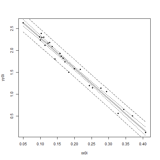

例2.4 年齢と最高血圧(pp.75-82)その1
5つのモデルについて、lm関数を使用して回帰パラメーターを推定したところまで。
> dtf <- read.csv("data/table2_5.csv", header = TRUE)
> xxi <- as.double(dtf$AGE)
> yyi <- as.double(dtf$BP)
> # (AGE, BP)
> r <- lm(yyi ~ 1 + xxi)
> print(r)
Call:
lm(formula = yyi ~ 1 + xxi)
Coefficients:
(Intercept)          xxi
   112.3167       0.4451
> # (AGE, log(BP))
> r <- lm(log(yyi) ~ 1 + xxi)
> print(r)
Call:
lm(formula = log(yyi) ~ 1 + xxi)
Coefficients:
(Intercept)          xxi
   4.732231     0.003365
> # (log(AGE), log(BP))
> r <- lm(log(yyi) ~ 1 + log(xxi))
> print(r)
Call:
lm(formula = log(yyi) ~ 1 + log(xxi))
Coefficients:
(Intercept)     log(xxi)
      4.411        0.127
> # (AGE^2 / 10000, log(BP))
> r <- lm(log(yyi) ~ 1 + I(xxi ^ 2 / 10000))
> print(r)
Call:
lm(formula = log(yyi) ~ 1 + I(xxi^2/10000))
Coefficients:
   (Intercept)  I(xxi^2/10000)
        4.7942          0.3863
> # (AGE^1.825 / 10000, log(BP))
> r <- lm(log(yyi) ~ 1 + I(xxi ^ 1.825 / 10000))
> print(r)
Call:
lm(formula = log(yyi) ~ 1 + I(xxi^1.825/10000))
Coefficients:
       (Intercept)  I(xxi^1.825/10000)
            4.7883              0.8272
例3.3 配達時間 (1),(2)(pp.106-113)
式(3.62)のモデルで計算している。表3.2(p.112)の対数尤度などは完全に一致しない。書籍では、途中で値を切り捨てて計算をしているからだと思われる。
> dtf <- read.csv("table3_1.csv", header = TRUE)
> n <- nrow(dtf)
> xx2i <- as.double(dtf$CASE)
> xx3i <- as.double(dtf$DIS) ^ 2 / 1.e5
> yyi <- as.double(dtf$DVT)
> k <- 3
> mxy <- matrix(yyi, ncol = 1)
> mxxx <- matrix(c(rep(1., n), xx2i, xx3i), ncol = 3)
> mxbh <- solve(t(mxxx) %*% mxxx) %*% t(mxxx) %*% mxy
> mxyh <- mxxx %*% mxbh
> mxe <- mxy - mxyh
> ssy2 <- sum(t(mxy) %*% mxy) - sum(yyi) ^ 2 / n
> ssyh2 <- sum(t(mxyh) %*% mxyh) - sum(yyi) ^ 2 / n
> sse2 <- as.vector(t(mxe) %*% mxe)
> s2 <- sse2 / (n - k)
> s <- sqrt(s2)
> mxvv <- s2 * solve(t(mxxx) %*% mxxx)
> mxs <- sqrt(diag(mxvv))
> rr2 <- ssyh2 / ssy2
> rrb2 <- 1 - (n - 1) / (n - k) * (1 - rr2)
> tbh <- as.vector(mxbh / mxs)
> sh2 <- sse2 / n
> logll <- -n / 2 * log(2 * pi) - n / 2 * log(sh2) - sse2 / (2 * sh2)
> p <- k + 1
> aic <- -2 * logll + 2 * p
> sbic <- -2 * logll + p * log(n)
> gcv <- -2 * logll - 2 * n * log(1 - p / n)
> hq <- -2 * logll + 2 * p * log(log(n))
> yyhi <- as.vector(mxyh)
> ei <- yyi - yyhi
> ri <- ei / yyi * 100
> ai2 <- ei ^ 2 / sum(ei ^ 2) * 100
> #
> cat("求めた回帰係数 β\n")
求めた回帰係数 β
> print(mxbh)
         [,1]
[1,] 6.191398
[2,] 1.410930
[3,] 1.424706
> cat("回帰係数の標準誤差 s\n")
回帰係数の標準誤差 s
> print(mxs)
[1] 0.8673945 0.1276345 0.1992415
> cat("仮説を検定するためのt値\n")
仮説を検定するためのt値
> print(tbh)
[1]  7.137927 11.054459  7.150648
> cat(sprintf("R^2   = %8.4f\n", rr2))
R^2   =   0.9791
> cat(sprintf("R~^2  = %8.4f\n", rrb2))
R~^2  =   0.9772
> cat(sprintf("log L = %8.4f\n", logll))
log L = -55.1821
> cat(sprintf("AIC   = %8.4f\n", aic))
AIC   = 118.3641
> cat(sprintf("SBIC  = %8.4f\n", sbic))
SBIC  = 123.2396
> cat(sprintf("GCV   = %8.4f\n", gcv))
GCV   = 119.0818
> cat(sprintf("HQ    = %8.4f\n", hq))
HQ    = 119.7164
> st <- sprintf("%5.2f %5.2f %5.2f %6.2f %5.2f", yyi, yyhi, ei, ri, ai2)
> for (i in 1:n) cat(sprintf("%2d %s\n", i, st[i]))
 1 16.68 20.54 -3.86 -23.12 12.29
 2 11.50 11.11  0.39   3.36  0.12
 3 12.03 12.07 -0.04  -0.34  0.00
 4 14.88 11.93  2.95  19.85  7.21
 5 13.75 14.98 -1.23  -8.93  1.25
 6 18.11 17.62  0.49   2.71  0.20
 7  8.00  9.19 -1.19 -14.82  1.16
 8 17.83 16.70  1.13   6.36  1.06
 9 79.24 78.89  0.35   0.44  0.10
10 21.50 18.46  3.04  14.14  7.64
11 40.33 35.51  4.82  11.95 19.20
12 21.00 20.96  0.04   0.19  0.00
13 13.50 12.76  0.74   5.47  0.45
14 19.75 17.70  2.05  10.39  3.48
15 24.00 21.75  2.25   9.38  4.19
16 29.00 28.88  0.12   0.41  0.01
17 15.35 15.23  0.12   0.80  0.01
18 19.00 16.32  2.68  14.13  5.95
19  9.50 10.44 -0.94  -9.92  0.73
20 35.10 38.62 -3.52 -10.04 10.27
21 17.90 20.58 -2.68 -14.97  5.94
22 52.32 52.22  0.10   0.19  0.01
23 18.75 21.77 -3.02 -16.13  7.56
24 19.83 23.22 -3.39 -17.11  9.52
25 10.75 12.16 -1.41 -13.08  1.63
例3.3 配達時間 (1),(2)(pp.106-113)※lm関数使用版
> dtf <- read.csv("table3_1.csv", header = TRUE)
> n <- nrow(dtf)
> xx2i <- as.double(dtf$CASE)
> xx3i <- as.double(dtf$DIS) ^ 2 / 1.e5
> yyi <- as.double(dtf$DVT)
> #
> r <- lm(yyi ~ xx2i + xx3i)
> sr <- summary(r)
> # 求めた回帰係数β,回帰係数の標準誤差s,仮説を検定するためのt値,p値
> print(sr$coef)
            Estimate Std. Error   t value     Pr(>|t|)
(Intercept) 6.191398  0.8673945  7.137927 3.711853e-07
xx2i        1.410930  0.1276345 11.054459 1.890317e-10
xx3i        1.424706  0.1992415  7.150648 3.609898e-07
> # R^2
> print(sr$r.squared)
[1] 0.9790869
> # R~^2
> print(sr$adj.r.squared)
[1] 0.9771857
> # log L
> print(logLik(r))
'log Lik.' -55.18207 (df=4)
> # AIC
> print(AIC(r))
[1] 118.3641
> # SBIC
> print(BIC(r))
[1] 123.2396
例3.3 配達時間 (3)(pp.113-114)
簡略化のため、lm関数を使用して計算している。
> dtf <- read.csv("table3_1.csv", header = TRUE)
> xx2i <- dtf$CASE
> xx3i <- dtf$DIS ^ 2 / 1.e5
> yyi <- dtf$DVT
> # (3.64)式
> r <- lm(yyi[-c(11)] ~ xx2i[-c(11)] + xx3i[-c(11)])
> print(summary(r))
Call:
lm(formula = yyi[-c(11)] ~ xx2i[-c(11)] + xx3i[-c(11)])
Residuals:
    Min      1Q  Median      3Q     Max
-3.8002 -1.2991  0.3215  1.3196  3.0112
Coefficients:
             Estimate Std. Error t value Pr(>|t|)
(Intercept)    6.4226     0.7920   8.110 6.62e-08 ***
xx2i[-c(11)]   1.3376     0.1196  11.182 2.65e-10 ***
xx3i[-c(11)]   1.4969     0.1831   8.178 5.78e-08 ***
---
Signif. codes:  0 ‘***’ 0.001 ‘**’ 0.01 ‘*’ 0.05 ‘.’ 0.1 ‘ ’ 1
Residual standard error: 2.125 on 21 degrees of freedom
Multiple R-squared:  0.9826,    Adjusted R-squared:  0.9809
F-statistic: 592.7 on 2 and 21 DF,  p-value: < 2.2e-16
> # (3.66)式
> ddi <- rep(0., nrow(dtf))
> ddi[11] <- 1
> r <- lm(yyi ~ xx2i + xx3i + ddi)
> print(summary(r))
Call:
lm(formula = yyi ~ xx2i + xx3i + ddi)
Residuals:
   Min     1Q Median     3Q    Max
-3.800 -1.279  0.303  1.298  3.011
Coefficients:
            Estimate Std. Error t value Pr(>|t|)
(Intercept)   6.4226     0.7920   8.110 6.62e-08 ***
xx2i          1.3376     0.1196  11.182 2.65e-10 ***
xx3i          1.4969     0.1831   8.178 5.78e-08 ***
ddi           5.4200     2.2536   2.405   0.0255 *
---
Signif. codes:  0 ‘***’ 0.001 ‘**’ 0.01 ‘*’ 0.05 ‘.’ 0.1 ‘ ’ 1
Residual standard error: 2.125 on 21 degrees of freedom
Multiple R-squared:  0.9836,    Adjusted R-squared:  0.9813
F-statistic: 419.9 on 3 and 21 DF,  p-value: < 2.2e-16
例3.4 平均勤続年数と所定内賃金(pp.116-118)
lm関数を使って計算している。以下に表示している表3.4(p.116)の値をCSV形式で入力したtable3_4.csvをカレントディレクトリに置いておくこと。
i,     W, YEAR, DX
 1, 209.0,  0.3,  1
 2, 237.0,  2.0,  1
 3, 301.7,  5.9,  1
 4, 371.6, 10.1,  1
 5, 455.3, 14.9,  1
 6, 526.6, 20.9,  1
 7, 579.9, 25.4,  1
 8, 587.3, 29.3,  1
 9, 477.0, 33.8,  1
10, 201.7,  0.3,  0
11, 228.7,  2.6,  0
12, 271.5,  6.3,  0
13, 308.1,  9.8,  0
14, 342.7, 14.5,  0
15, 389.0, 20.0,  0
16, 394.6, 23.8,  0
17, 399.8, 28.3,  0
18, 317.0, 32.6,  0
> dtf <- read.csv("table3_4.csv", header = TRUE)
> xx1i <- as.double(dtf$YEAR)
> xx2i <- as.double(dtf$DX)
> yyi <- as.double(dtf$W)
> r <- lm(yyi ~ 1 + log(xx1i) + I(xx1i ^ 2) + I(xx1i ^ 4) + I(xx2i * xx1i))
> print(summary(r))
Call:
lm(formula = yyi ~ 1 + log(xx1i) + I(xx1i^2) + I(xx1i^4) + I(xx2i *
xx1i))
Residuals:
Min 1Q Median 3Q Max
-17.136 -7.683 2.097 7.070 17.824
Coefficients:
Estimate Std. Error t value Pr(>|t|)
(Intercept) 2.196e+02 4.748e+00 46.26 8.20e-16 ***
log(xx1i) 1.469e+01 3.257e+00 4.51 0.000586 ***
I(xx1i^2) 5.088e-01 3.531e-02 14.41 2.27e-09 ***
I(xx1i^4) -4.446e-04 2.817e-05 -15.78 7.36e-10 ***
I(xx2i * xx1i) 6.523e+00 2.722e-01 23.96 3.84e-12 ***
---
Signif. codes: 0 ‘***’ 0.001 ‘**’ 0.01 ‘*’ 0.05 ‘.’ 0.1 ‘ ’ 1
Residual standard error: 11.01 on 13 degrees of freedom
Multiple R-squared: 0.9937, Adjusted R-squared: 0.9917
F-statistic: 511.7 on 4 and 13 DF, p-value: 3.746e-14
> yyhi <- r$fitted.value
> ei <- yyi - yyhi
> ri <- ei / yyi * 100
> ai2 <- ei ^ 2 / sum(ei ^ 2) * 100
> dtf <- data.frame(yyi, xx1i, yyhi, ei, ri, ai2)
> names(dtf) <- c("W", "YEAR", "Wの推定値", "残差", "誤差率", "平方残差率")
> print(dtf)
W YEAR Wの推定値 残差 誤差率 平方残差率
1 209.0 0.3 203.9620 5.0379825 2.4105179 1.609669358
2 237.0 2.0 244.9042 -7.9041701 -3.3350929 3.962195699
3 301.7 5.9 301.3806 0.3194241 0.1058747 0.006470811
4 371.6 10.1 366.7761 4.8238794 1.2981376 1.475761750
5 455.3 14.9 447.5628 7.7372332 1.6993704 3.796599095
6 526.6 20.9 538.0347 -11.4347032 -2.1714210 8.292264754
7 579.9 25.4 576.0246 3.8753715 0.6682827 0.952467251
8 587.3 29.3 569.4762 17.8237961 3.0348708 20.147621237
9 477.0 33.8 492.7775 -15.7775142 -3.3076550 15.787033282
10 201.7 0.3 202.0051 -0.3050563 -0.1512426 0.005901786
11 228.7 2.6 237.1031 -8.4031158 -3.6742964 4.478205967
12 271.5 6.3 266.1784 5.3215546 1.9600569 1.795975490
13 308.1 9.8 297.9372 10.1627947 3.2985377 6.550126198
14 342.7 14.5 346.2444 -3.5444215 -1.0342636 0.796735341
15 389.0 20.0 396.0212 -7.0212080 -1.8049378 3.126418007
16 394.6 23.8 411.7361 -17.1361000 -4.3426508 18.622901255
17 399.8 28.3 391.0281 8.7718944 2.1940706 4.879891365
18 317.0 32.6 309.3476 7.6523586 2.4139932 3.713761354貨幣賃金率変化率の回帰モデルの推定(pp.119-120)
表3.7の値をCSV形式で入力したtable3_7.csvをカレントディレクトリに置いておく。
> dtf <- read.csv("table3_7.csv", header = TRUE)
> xx1i <- 1 / as.double(dtf$RU)
> xx2i <- as.double(dtf$CPIDOT)
> yyi <- as.double(dtf$WDOT)
> n <- length(xx1i)
> k <- 3
> degf <- n - k
> mxy <- matrix(yyi, ncol = 1)
> mxxx <- matrix(c(rep(1.0, n), xx1i, xx2i), ncol = 3)
> mxxxtxxi <- solve(t(mxxx) %*% mxxx)
> mxbh <- mxxxtxxi %*% t(mxxx) %*% mxy
> mxyh <- mxxx %*% mxbh
> mxe <- mxy - mxyh
> sse2 <- t(mxe) %*% mxe
> s2 <- as.vector(sse2 / degf)
> s <- sqrt(s2)
> mxvv <- s2 * mxxxtxxi
> mxs <- matrix(sqrt(diag(mxvv)), ncol = 1)
> tj <- as.vector(mxbh / mxs)
> pj <- 2 * pt(abs(tj), degf, lower.tail = FALSE)
> bh <- as.vector(mxbh)
> yyhi <- as.vector(mxyh)
> ei <- yyi - yyhi
> yym <- mean(yyi)
> rr2 <- sum((yyhi - yym) ^ 2) / sum((yyi - yym) ^ 2)
> rrb2 <- 1 - (n - 1) / (n - k) * (1 - rr2)
> print(bh)  # 推定した回帰モデルのパラメーター
[1] -4.6884718 16.2320984  0.8915398
> print(tj)  # t値
[1] -8.938476 12.501712 12.623158
> print(pj)  # p値
[1] 6.096213e-12 5.248937e-17 3.628214e-17
> print(rr2)  # 決定係数
[1] 0.9509842
> print(rrb2)  # 自由度修正済み決定係数
[1] 0.9490236
> print(s)  # 誤差項の分散の不偏推定量の標準誤差
[1] 1.580779