R入門
Rによるセイバーメトリクス入門(技術評論社)
最終更新:
r-intro
-
view
目次
1960年代に最も多くホームランを放ったプレイヤー(pp.58-59)
> library(Lahman)
> library(tidyverse)
> Batting %>% filter(yearID >= 1960, yearID <= 1969) -> Batting_60
> Batting_60 %>% group_by(playerID) %>% summarize(HR = sum(HR)) -> hr_60
> hr_60 %>% arrange(desc(HR)) -> hr_60
> print(head(hr_60))
# A tibble: 6 × 2
  playerID     HR
  <chr>     <int>
1 killeha01   393
2 aaronha01   375
3 mayswi01    350
4 robinfr02   316
5 mccovwi01   300
6 howarfr01   288
10年ごとに最も多くホームランを放ったプレイヤー(pp.59-61)
> library(Lahman)
> library(tidyverse)
> hr_leader <- function(data) {
+ data %>% group_by(playerID) %>% summarize(HR = sum(HR)) %>%
+ arrange(desc(HR)) %>% head(1)
+ }
> Batting %>% mutate(decade = 10 * floor(yearID / 10)) %>%
+ split(pull(., decade)) %>% map_df(hr_leader, .id = "decade")
# A tibble: 16 × 3
   decade playerID     HR
   <chr>  <chr>     <int>
 1 1870   pikeli01     21
 2 1880   stoveha01    89
 3 1890   duffyhu01    83
 4 1900   davisha01    67
 5 1910   cravaga01   116
 6 1920   ruthba01    467
 7 1930   foxxji01    415
 8 1940   willite01   234
 9 1950   snidedu01   326
10 1960   killeha01   393
11 1970   stargwi01   296
12 1980   schmimi01   313
13 1990   mcgwima01   405
14 2000   rodrial01   435
15 2010   cruzne02    346
16 2020   perezsa02    59
5,000打数以上経験した全プレイヤーの三振率とホームラン率(pp.61-63)
> library(Lahman)
> library(tidyverse)
> library(ggplot2)
> Batting %>% group_by(playerID) %>%
+ summarize(tAB = sum(AB, na.rm = TRUE),
+   tHR = sum(HR, na.rm = TRUE),
+   tSO = sum(SO, na.rm = TRUE)) -> long_careers
> Batting_5000 <- filter(long_careers, tAB >= 5000)
> print(head(Batting_5000))
# A tibble: 6 × 4
  playerID    tAB   tHR   tSO
  <chr>     <int> <int> <int>
1 aaronha01 12364   755  1383
2 abreubo01  8480   288  1840
3 adamssp01  5557     9   223
4 adcocjo01  6606   336  1059
5 alfoned01  5385   146   617
6 allendi01  6332   351  1556
> g <- ggplot(Batting_5000, aes(x = tHR / tAB, y = tSO / tAB)) +
+ geom_point() + geom_smooth()
> print(g)
`geom_smooth()` using method = 'loess' and formula = 'y ~ x'
imageプラグインエラー : ご指定のファイルが見つかりません。ファイル名を確認して、再度指定してください。 (fig2_9.png)
MLBにおける2001~2010年の得点差分と勝率の散布図(pp.95-99)
> library(tidyverse)
> library(Lahman)
> my_teams <- Teams %>% filter(yearID > 2000 & yearID < 2011) %>%
+ select(teamID, yearID, lgID, G, W, L, R, RA)
> my_teams %>% tail()
    teamID yearID lgID   G  W  L   R  RA
295    SFN   2010   NL 162 92 70 697 583
296    SLN   2010   NL 162 86 76 736 641
297    TBA   2010   AL 162 96 66 802 649
298    TEX   2010   AL 162 90 72 787 687
299    TOR   2010   AL 162 85 77 755 728
300    WAS   2010   NL 162 69 93 655 742
> my_teams <- my_teams %>% mutate(RD = R - RA, Wpct = W / (W + L))
> run_diff <- ggplot(my_teams, aes(x = RD, y = Wpct)) + geom_point() +
+ scale_x_continuous("Run differential") +
+ scale_y_continuous("Winning percentage")
> print(run_diff)
> crcblue <- "#2905A1"
> linfit <- lm(Wpct ~ RD, data = my_teams)
> print(linfit)
Call:
lm(formula = Wpct ~ RD, data = my_teams)
Coefficients:
(Intercept)           RD
  0.4999909    0.0006216
> run_diff + geom_smooth(method = "lm", se = FALSE, color = crcblue)
`geom_smooth()` using formula = 'y ~ x'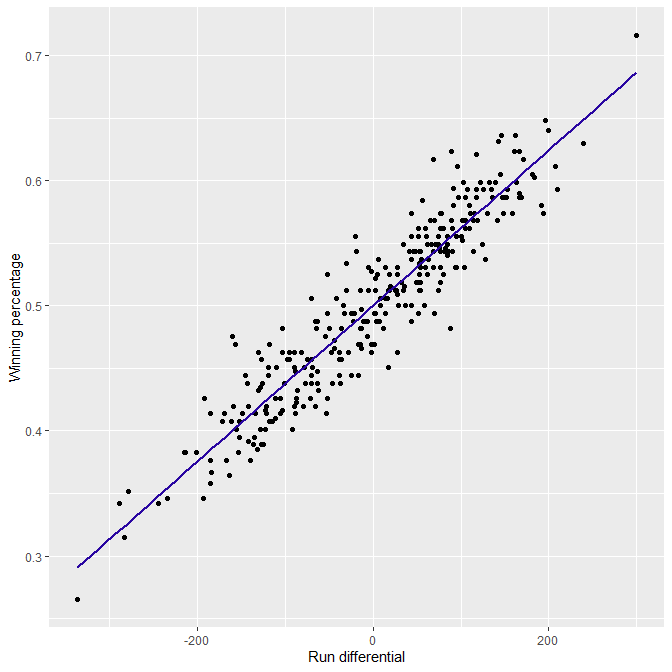
Mickey Mantleの打撃成績推移(pp.184-188)
> library(tidyverse)
> library(Lahman)
> get_stats <- function(player.id) {
+ batting %>%
+ filter(playerID == player.id) %>%
+ inner_join(People, by = "playerID") %>%
+ mutate(birthyear = ifelse(birthMonth >= 7, birthYear + 1,
+   birthYear),
+    Age = yearID - birthyear,
+    SLG = (H - X2B - X3B - HR + 2 * X2B + 3 * X3B + 4 * HR) / AB,
+    OBP = (H + BB + HBP) / (AB + BB + HBP + SF),
+    OPS = SLG + OBP) %>%
+ select(Age, SLG, OBP, OPS)
+ }
> fit_model <- function(d) {
+ fit <- lm(OPS ~ I(Age - 30) + I((Age - 30) ^ 2), data = d)
+ b <- coef(fit)
+ Age.max <- 30 - b[2] / b[3] / 2
+ Max <- b[1] - b[2] ^ 2 / b[3] / 4
+ list(fit = fit, Age.max = Age.max, Max = Max)
+ }
> People %>%
+ filter(nameFirst == "Mickey", nameLast == "Mantle") %>%
+ pull(playerID) -> mantle_id
> Batting %>% replace_na(list(SF = 0, HBP = 0)) -> batting
> Mantle <- get_stats(mantle_id)
> g8_1 <- ggplot(Mantle, aes(Age, OPS)) + geom_point()
> ggsave("fig8_1.png", plot = g8_1)
Saving 7 x 7 in image
> F2 <- fit_model(Mantle)
> print(coef(F2$fit))
    (Intercept)     I(Age - 30) I((Age - 30)^2)
    1.043134189    -0.022883024    -0.003868915
> print(c(F2$Age.max, F2$Max))
I(Age - 30) (Intercept)
   27.04271     1.07697
> g8_2 <- ggplot(Mantle, aes(Age, OPS)) + geom_point() +
+ geom_smooth(method = "lm", se = FALSE, size = 1.5,
+ formula = y ~ poly(x, 2, raw= TRUE)) +
+ geom_vline(xintercept = F2$Age.max, linetype = "dashed",
+    color = "darkgrey") +
+ geom_hline(yintercept = F2$Max, linetype = "dashed", color = "darkgrey") +
+ annotate(geom = "text", x = c(29, 20), y = c(0.72, 1.1),
+  label = c("Peak age", "Max"), size = 5)
> ggsave("fig8_2.png", plot = g8_2)
Saving 7 x 7 in image
> print(F2 %>% pluck("fit") %>% summary())
Call:
lm(formula = OPS ~ I(Age - 30) + I((Age - 30)^2), data = d)
Residuals:
     Min       1Q   Median       3Q      Max
-0.17282 -0.04010  0.02203  0.04507  0.12819
Coefficients:
                  Estimate Std. Error t value Pr(>|t|)
(Intercept)      1.0431342  0.0279009  37.387 3.19e-16 ***
I(Age - 30)     -0.0228830  0.0056381  -4.059 0.001029 **
I((Age - 30)^2) -0.0038689  0.0008283  -4.671 0.000302 ***
---
Signif. codes:  0 ‘***’ 0.001 ‘**’ 0.01 ‘*’ 0.05 ‘.’ 0.1 ‘ ’ 1
Residual standard error: 0.08421 on 15 degrees of freedom
Multiple R-squared:  0.6018,    Adjusted R-squared:  0.5488
F-statistic: 11.34 on 2 and 15 DF,  p-value: 0.001001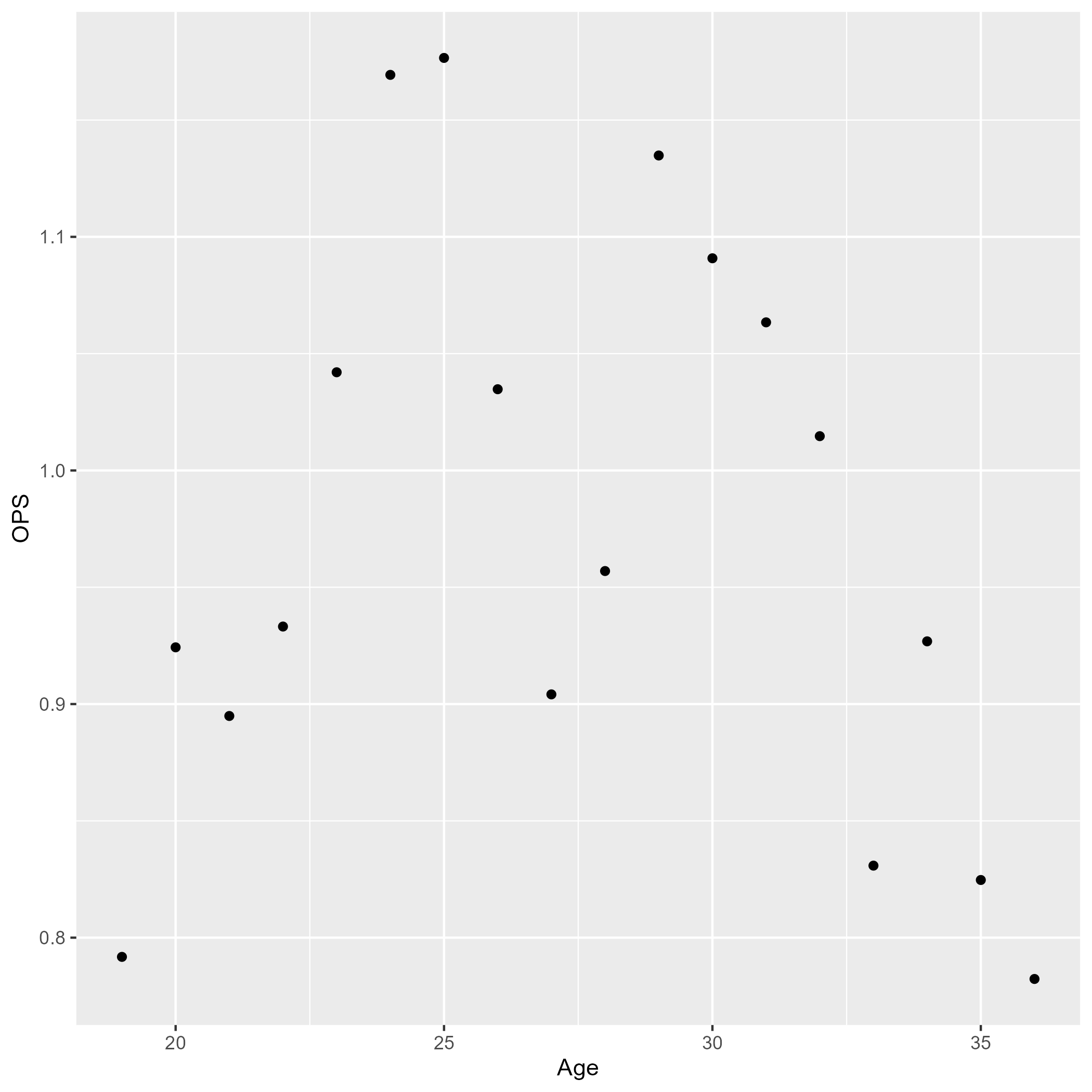
cwevent.exeの出力フィールドのヘッダー一覧をベクトルで得る
cwevent.exeの出力するフィールド情報は、以下のページで公開されている。 https://chadwick.sourceforge.net/doc/cwevent.html このページ内の表にそれぞれ標準フィールド(全97個)と拡張フィールド(62個)が示されており、rvestパッケージのread_html関数とhtml_table関数を使うことで、それぞれのフィールドのヘッダーを、文字列ベクトルで簡単に抜き出すことができる。
> library(rvest)
> html <- read_html("https://chadwick.sourceforge.net/doc/cwevent.html")
> tbl <- html_table(html, header = NA)
> s1 <- tbl[[1]]$Header
> s2 <- tbl[[2]]$Header
> print(s1)
 [1] "GAME_ID"                   "AWAY_TEAM_ID"
 [3] "INN_CT"                    "BAT_HOME_ID"
 [5] "OUTS_CT"                   "BALLS_CT"
(以下、表示省略)
> print(s2)
 [1] "HOME_TEAM_ID"           "BAT_TEAM_ID"
 [3] "FLD_TEAM_ID"            "BAT_LAST_ID"
 [5] "INN_NEW_FL"             "INN_END_FL"
(以下、表示省略)